This blog post was created for my PIC16B class at UCLA (Previously titled: Blog Post 5 - Distinguishing Between Cats and Dogs Ft. TensorFlow).

Distinguishing between cats and dogs seems like the easiest task in the world. And yet, training a machine learning model to do so is a non-trivial problem. As such, in this blog post, we will be learning several new skills, methods, and concepts related to image classification in TensorFlow, an open-source library for machine learning and artificial intelligence.

Acknowledgements

Many parts of this blog post, including chunks of code, are based on the TensorFlow Transfer Learning Tutorial.

Part 1: Loading Packages and Obtaining the Data

We will start be creating a block of code that will hold our import statements. Feel free to import any other packages you deem necessary!

import os
import tensorflow as tf
from tensorflow.keras import utils

As always, our first step in any data science/machine learning project is to acquire the data and load it into Python. We will be using a sample data set containing labeled images of cats and dogs, provided by the TensorFlow team.

By running the following block of code, we create a Tensorflow Dataset for training, validating, and testing our machine learning model(s). In this case, we use Datasets since it is not all that practical to load this data into memory.

# location of data
_URL = 'https://storage.googleapis.com/mledu-datasets/cats_and_dogs_filtered.zip'

# download the data and extract it
path_to_zip = utils.get_file('cats_and_dogs.zip', origin=_URL, extract=True)

# construct paths
PATH = os.path.join(os.path.dirname(path_to_zip), 'cats_and_dogs_filtered')

train_dir = os.path.join(PATH, 'train')
validation_dir = os.path.join(PATH, 'validation')

# parameters for datasets
BATCH_SIZE = 32
IMG_SIZE = (160, 160)

# construct train and validation datasets 
train_dataset = utils.image_dataset_from_directory(train_dir,
                                                   shuffle=True,
                                                   batch_size=BATCH_SIZE,
                                                   image_size=IMG_SIZE)

validation_dataset = utils.image_dataset_from_directory(validation_dir,
                                                        shuffle=True,
                                                        batch_size=BATCH_SIZE,
                                                        image_size=IMG_SIZE)

# extracting the class names
class_names = train_dataset.class_names

# construct the test dataset by taking every 5th observation out of the validation dataset
val_batches = tf.data.experimental.cardinality(validation_dataset)
test_dataset = validation_dataset.take(val_batches // 5)
validation_dataset = validation_dataset.skip(val_batches // 5)

Notice that we have used a special-purpose keras utility that constructs a Dataset called image_dataset_from_directory. The first, and arguably the most important argument, of this utility states where the images are located (i.e., the path to the images). The shuffle argument set to True ensures that data received from the directory is randomized. The batch_size determines how many data points are gathered from the directory at once. For instance, in the above chunk of code, we have set our BATCH_SIZE=32 which means that each time we request some data, we will get 32 images from each of the data sets. Finally, as the name suggests, the image_size set to (160, 160) defines the size of the input images.

Now that we’ve done that, the next chunk of code rapidly reads the data! The execution time is sped up since tf.data.AUTOTUNE prompts the tf.data runtime to tune the value dynamically at runtime!

AUTOTUNE = tf.data.AUTOTUNE

train_dataset = train_dataset.prefetch(buffer_size=AUTOTUNE)
validation_dataset = validation_dataset.prefetch(buffer_size=AUTOTUNE)
test_dataset = test_dataset.prefetch(buffer_size=AUTOTUNE)

Working with Datasets

Now that we’ve acquired the data, let’s go ahead and briefly explore it! We will be writing a function that creates a two-row, three-column visualization of the dogs and cats. Our first row will consist of cats while the second will have dogs. The objective here is to see whether we can successfully retrieve a piece of the data using the .take() method.

Before writing our function, let’s go ahead and import a couple of other packages (matplotlib, numpy, random) in our import code block (above):

import os
import tensorflow as tf
from tensorflow.keras import utils
from matplotlib import pyplot as plt
import numpy as np
import random

Now that we’ve done that, we can go ahead and write our visualization function.

def visualize_cats_and_dogs():
    """
    Function generates a two-row, three-column
    visualization of dogs and cats
    """
    plt.figure(figsize=(15, 10)) #size of our visualization
    for images, labels in train_dataset.take(1):
        cnum = 0 # number of cats
        dnum = 0 # number of dogs
        cats = [] # list of index positions of cats
        dogs = [] # list of index positions of dogs
        for i in range(len(labels)):
            if class_names[labels[i]] == "cat":
                # Append the index position i to the cats list
                # if the label == cat
                cats.append(i)
            else:
                # If the label == dog
                # Append the index position i to the dogs list
                dogs.append(i)
        # randomly select three random cats and dogs from the
        # respective lists
        rand_cats = random.sample(cats, 3)
        rand_dogs = random.sample(dogs, 3)
        # Joining the two lists
        cats_and_dogs = rand_cats + rand_dogs

        for i in cats_and_dogs:
            # checking if cat
            if class_names[labels[i]] == "cat":
                if cnum >= 3:
                    # We are checking if the cat number is greater than 3
                    # if it is, continue the loop without performing
                    # any tasks
                    continue
                ax = plt.subplot(2, 3, cnum+1)
                plt.imshow(images[i].numpy().astype("uint8"))
                plt.title("cats")
                plt.axis("off")
                cnum += 1
            else:
                if dnum >= 3:
                    # We are checking if the dog number is greater than 3
                    # if it is, continue the loop without performing
                    # any tasks
                    continue
                ax = plt.subplot(2, 3, dnum+4)
                plt.imshow(images[i].numpy().astype("uint8"))
                plt.title("dogs")
                plt.axis("off")
                dnum += 1

Now that we’ve defined our function, let’s test it to see if it works!

visualize_cats_and_dogs()

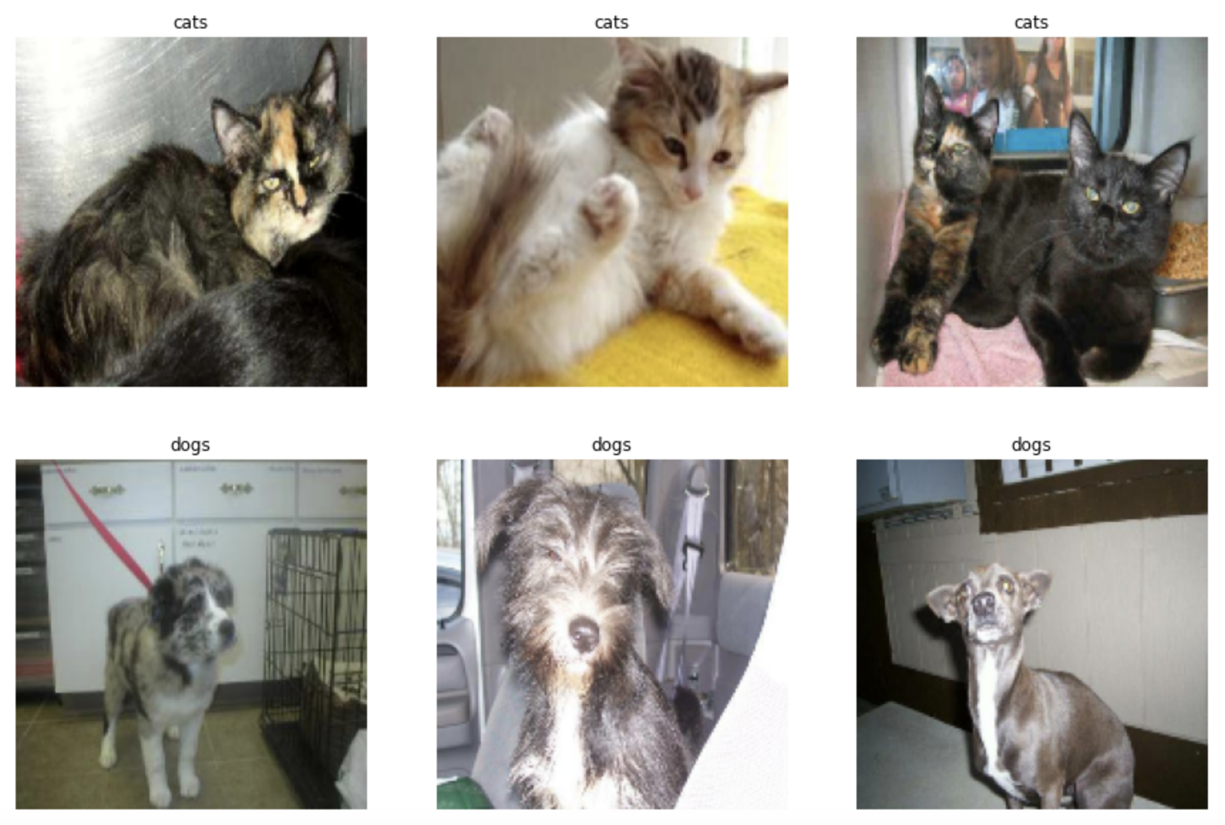
Hooray, our function worked! Look at all of those cute cats and dogs!

Checking the Label Frequencies

The following code creates an iterator called labels_iterator.

labels_iterator= train_dataset.unbatch().map(lambda image, label: label).as_numpy_iterator()

We would like to compute the number of images in our training data with label 0 (cats) and label 1 (dogs). Why do we care about this? We need to know the most frequent label since our baseline machine learning model is likely to guess that label!

To find the number of labels corresponding to 0, we simple take the sum of the iterator.

sum(labels_iterator)

1000

Since we have a total of 2000 images, we automatically realize that the number of labels corresponding to 1 is also 1000. We can then compute the accuracy of our baseline machine learning model!

baseline = 1000/2000

print(baseline)

0.5

So, the baseline accuracy of our model is 0.5! Going forward, we will treat this as a benchmark for improvement.

Part 2: First Model

You probably already know that this image classification problem involves assigning a labels to images. In this case, we have several images of cats and dogs and want to assign the “cat” or “dog” label to the appropriate images. One of the most important tools for image classification is most convolutional neural networks (CNNs).

Convolution can be used to extract features from images. But, what is convolution exactly?
In mathematics, convolution is a mathematical operation on two functions that produces an output function that expresses how the shape of one of those functions was modified by the other function. In machine learning, we are likely to have matrices of input data. So, the idea of convolution is that we define a kernel matrix and “slide it over” the input data, resulting in an output matrix describing how the input matrix was modifed by the kernel matrix!

There are many different possibilities of convolutional kernels we could “slide over” the input data. In practice, we treat these kernels as parameters and learn them from our input data as part of the model fitting process. This is what the Conv2D layer allows us to do within our tf.keras.Sequential model. The MaxPooling2D layers act as summary layers that reduce the size of the data at each step. While building our model we will be following the common approach and alternating between Conv2D and MaxPooling2D.

After the series of Conv2D and MaxPooling2D layers, we will need to Flatten the data from its current 2D shape to a 1D shape, allowing it to pass through to the final Dense layer(s). The Dense layers perform the classification.

Dropout is an effective and commonly used regularization technique for convolutional neural networks. After applying it to a layer, we see our model randomly “dropping out” (i.e. setting the input to zero) a number of output features of the layer during training. The is key in reducing “overfitting” and thus, our Dropout layers should be placed before our Dense layers that form the prediction.

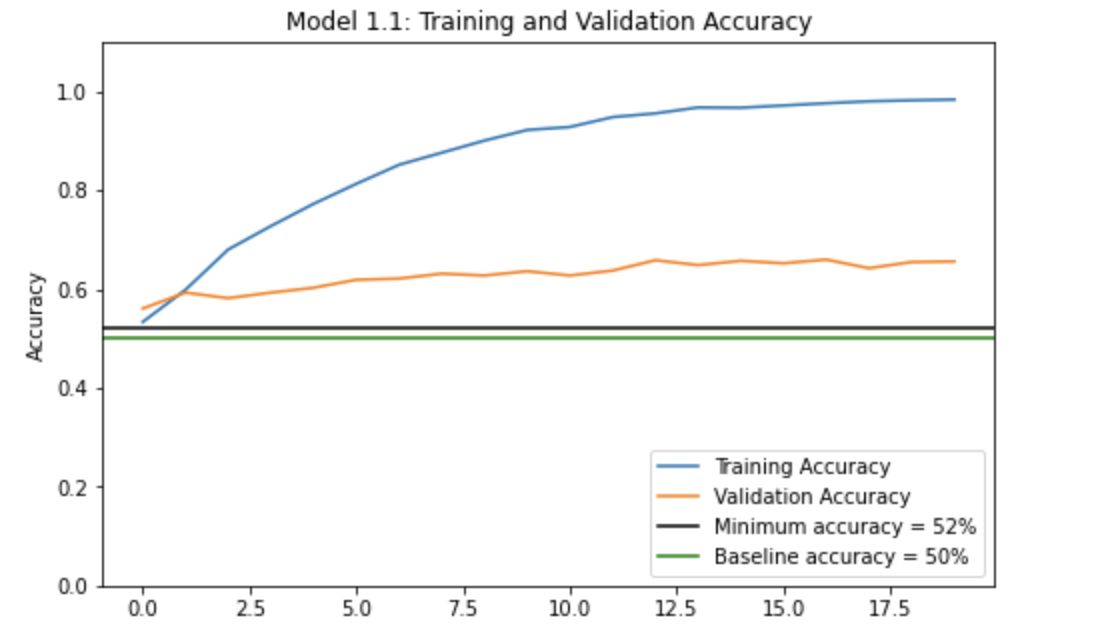
Keeing this in mind, we will create a tf.keras.Sequential model, call it model1, with at least two Conv2D and MaxPooling2D layer pairs, at least one Flatten, Dense, and Dropout respectively. After training our model, we will plot the history of the accuracy on both the training and validation sets.

Remember to import the required packages for your model!

from tensorflow.keras import layers
from tensorflow.keras import models

Model 1.1

Let’s create our model!

model1 = models.Sequential([
    layers.Conv2D(32, (3, 3), activation='relu', input_shape=(160, 160, 3)),
    layers.MaxPooling2D((2, 2)),
    layers.Conv2D(32, (3, 3), activation='relu'),
    layers.MaxPooling2D((2, 2)),
    layers.Flatten()
    layers.Dropout(0.2),
    layers.Dense(1)
])

Now that we have created our model, let’s get a summary of the above.

model1.summary()

Model: "sequential"
_________________________________________________________________
Layer (type)                Output Shape              Param #   
=================================================================
conv2d (Conv2D)             (None, 158, 158, 32)      896       
                                                             
 max_pooling2d (MaxPooling2D  (None, 79, 79, 32)       0         
)                                                               

conv2d_1 (Conv2D)           (None, 77, 77, 32)        9248      

max_pooling2d_1 (MaxPooling  (None, 38, 38, 32)       0         
2D)                                                             

flatten (Flatten)           (None, 46208)             0         

dropout (Dropout)           (None, 46208)             0         
                                                             
dense (Dense)               (None, 1)                 46209     
                                                             
=================================================================
Total params: 56,353
Trainable params: 56,353
Non-trainable params: 0
_________________________________________________________________

Now, let’s train our model!

base_learning_rate = 0.0001
model1.compile(optimizer=tf.keras.optimizers.Adam(learning_rate=base_learning_rate),
              loss=tf.keras.losses.BinaryCrossentropy(from_logits=True),
              metrics=['accuracy'])

history = model1.fit(train_dataset, 
                     epochs=20, 
                     validation_data=validation_dataset)

After 20 epochs, our training set accuracy reached 98.35% whereas our validation accuracy reached 65.59%. Let’s plot the history of the accuracy to get a better idea of what happened!

train_acc = history.history['accuracy']
val_acc = history.history['val_accuracy']

plt.figure(figsize=(8, 5))
plt.plot(train_acc, label='Training Accuracy')
plt.plot(val_acc, label='Validation Accuracy')
plt.ylabel('Accuracy')
plt.axhline(y=0.52, color='black', label='Minimum accuracy = 52%')
plt.axhline(y=0.50, color='green', label='Baseline accuracy = 50%')
plt.legend(loc='lower right')
plt.ylim([0,1.1])
plt.title('Model 1.1: Training and Validation Accuracy')
plt.show()

Model 1.2

Let’s try and see if we can get a better validation accuracy. We will add an extra Conv2D and MaxPooling2D layer to our model (as depicted below).

model1 = models.Sequential([
    layers.Conv2D(32, (3, 3), activation='relu', input_shape=(160, 160, 3)),
    layers.MaxPooling2D((2, 2)),
    layers.Conv2D(32, (3, 3), activation='relu'),
    layers.MaxPooling2D((2, 2)),
    # Extra Conv2D and MaxPooling2D layers
    layers.Conv2D(32, (3, 3), activation='relu'),
    layers.MaxPooling2D((2, 2)),
    layers.Flatten(),
    layers.Dropout(0.2),
    layers.Dense(1)
])

We train this model the same we did in Model 1.1 and plotted the history of accuracy on training and validation sets. Let’s look at these plots to see how we did.

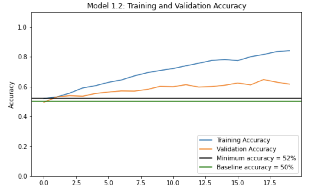
Looks like this time our validation accuracy reached only 61.63% and our training accuracy reached only 84.10%.

Model 1.3:

Let’s try another experiment! Let’s try adding in another Dense layer and see what happens:

model1 = models.Sequential([
    layers.Conv2D(32, (3, 3), activation='relu', input_shape=(160, 160, 3)),
    layers.MaxPooling2D((2, 2)),
    layers.Conv2D(32, (3, 3), activation='relu'),
    layers.MaxPooling2D((2, 2)),
    layers.Conv2D(32, (3, 3), activation='relu'),
    layers.MaxPooling2D((2, 2)),
    layers.Flatten(),
    # Additional dense layer added
    layers.Dense(64, activation='relu'),
    layers.Dropout(0.2),
    layers.Dense(1)
])

We train this model the same we did the other two and plotted the history of accuracy on training and validation sets. Once again, let’s see how we did.

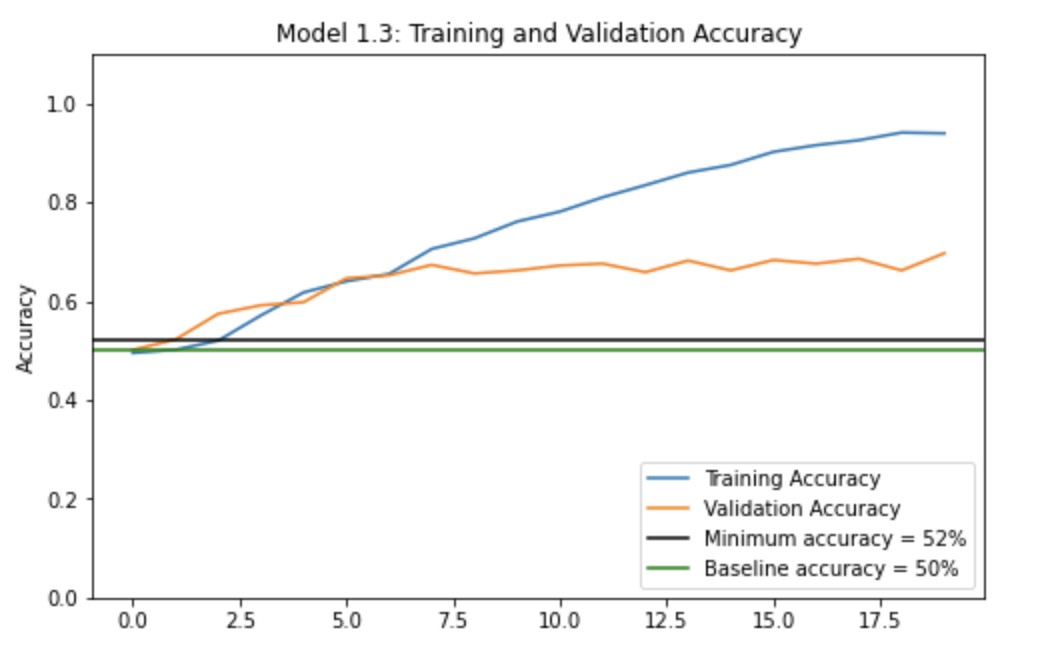
This time we reached a validation accuracy of 69.68%, the highest yet! Our training accuracy reached 93.95%

A number of experiments were conducted in a similar manner and we noticed that the validation accuracy seemed to stabilize between 60% and 70%. We consistently achieved about 10-15% better accuracy than the baseline = 50%, even better we consistently achieved at least a 52% validation accuracy.

Overfitting is typically observed when the training accuracy is much greater than the validation accuracy.
In all cases, the training accuracy was quite a bit greater than the validation accuracy; Models 1.1 and 1.3 in particular had a much higher training accuracies than validation accuracies. This indicates overfitting of the data.

Part 3: Model with Data Augmentation

When we do not have a large data set of images, we can try to artificially introduce diversity to the data set by applying random (but realistic) transformations to training images, like rotating the images or flipping them! This ultimately will help reduce overfitting, which was a major problem with our last model(s)!

Data augmentation refers to this practice of incorporating modified versions of the same image (like rotated or flipped images) in our training set. For example, an image of a cat is still going to be an image of a cat even if we flip it vertically or rotate it. We will include the transformed versions of these images in our training process to expose our model to different aspects of the training set.

Let’s first create a tf.keras.layers.RandomFlip() layer. Remember whether or not we flip the image of a dog or cat, it’s still the same image of the dog or cat! We will also make a plot of a randomly chosen image from the original data set and a few copies to which RandomFlip() have been applied. Let’s call our image flipping layer randomly_flip.

def randomly_flip = tf.keras.Sequential([
    # including the RandomFlip layer
    layers.RandomFlip('horizontal_and_vertical'),
])

Now, let’s make sure this layer works!

plt.figure(figsize=(15, 10))
for images, labels in train_dataset.take(1):
    img = images[0] # we want the first image
    img = tf.expand_dims(img, 0)
  
    for i in range(3):
        if i == 0:
            ax = plt.subplot(2, 3, i+1)
            plt.imshow(img[0] / 255)
            plt.axis('off')
            plt.title("Original Image")
        else:
            ax = plt.subplot(2, 3, i+1)
            aug_img = randomly_flip(img)
            plt.imshow(aug_img[0] / 255)
            plt.axis('off')
            plt.title("Randomly Flipped Image "+str(i))

Next, let’s create a tf.keras.layers.RandomRotation() layer. Remember whether or not we rotate the image of a dog or cat, it’s still the same image of a dog or cat! We will also make a plot of a randomly chosen image from the original data set and a few copies to which RandomRotation() have been applied. Let’s call our image rotating layer randomly_rotate.

randomly_rotate = tf.keras.Sequential([
    # Including the RandomRotation layer
    layers.RandomRotation(0.25),
])

Let’s check that our layer works!

plt.figure(figsize=(15, 10))
for images, labels in train_dataset.take(1):
    img = images[0] # we want the first image
    img = tf.expand_dims(img, 0)
  
    for i in range(3):
        if i == 0:
            ax = plt.subplot(2, 3, i+1)
            plt.imshow(img[0] / 255)
            plt.axis('off')
            plt.title("Original Image")
        else:
            ax = plt.subplot(2, 3, i+1)
            aug_img = randomly_rotate(img)
            plt.imshow(aug_img[0] / 255)
            plt.axis('off')
            plt.title("Randomly Rotated Image "+str(i))

Now that we’ve made sure that both of the above functions work, we can create a new tf.keras.models.Sequential model, call it model2, such that the first two layers are data augmentation layers! Let’s train this model (the same way did before) and visualize its training history.

model2 = models.Sequential([
    # Data Augmentation
    layers.RandomFlip("horizontal_and_vertical"),
    layers.RandomRotation(0.25),
    # Model 1.3:
    layers.Conv2D(32, (3, 3), activation='relu', input_shape=(160, 160, 3)),
    layers.MaxPooling2D((2, 2)),
    layers.Conv2D(32, (3, 3), activation='relu'),
    layers.MaxPooling2D((2, 2)),
    layers.Conv2D(32, (3, 3), activation='relu'),
    layers.MaxPooling2D((2, 2)),
    layers.Flatten(),
    layers.Dense(64, activation='relu'),
    layers.Dropout(0.2),
    layers.Dense(1)
])

We will train our model the same way we did earlier and plot the history of the accuracy!

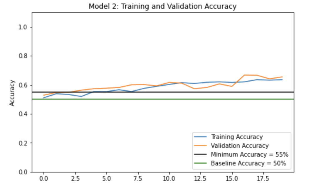
After ~2 epochs we consistently have a validation accuracy of above 55% (as shown in the above graph). Our validation accuracy also reaches 65.47%. The validation accuracy does not seem to stabilize during training, in fact the graph shows an upward trend, indicating that if the number of epochs were increased, it is possible that the validation accuracy would increase as well.

Compared to the validation accuracy of model1 (i.e., for Model 1.3 we achieved an accuracy of 69.68%), this validation accuracy is slightly lower. This might mean that our current model2 actually performs worse than model1.

However, though our validation accuracy for model2 is slightly lower than model1, we also note that the training accuracy is pretty comparable to the validation accuracy for model2. In fact, at around 15 epochs, we see that the validation accuracy surpasses the training accuracy! This implies that model2 most likely does not overfit the data.

Part 4: Data Processing

Making simple transformations to the input data can go a long way. We’ve already seen some transformations like flipping and rotating images (in Part 3), but what about the RGB values of the pixels? Currenly the pixels for our input data have RGB values between 0 and 255. However, models tend to train faster with RGB values normalized between the interval [0, 1] or even [-1, 1] - these are actually identical situations from a mathematical standpoint since all we have to do is scale the weights. By normalizing our RGB values in this way, we could minimize training energy need to have the weights adjust to the data scale and maximize training energy needed for handling the actual signal in the data!

The code block (below) will create a preprocessing layer called preprocessor which we will incorporate into our model pipeline.

i = tf.keras.Input(shape=(160, 160, 3))
x = tf.keras.applications.mobilenet_v2.preprocess_input(i)
preprocessor = tf.keras.Model(inputs = [i], outputs = [x])

Now, let’s go ahead and create model3 that incorporates the preprocesser!

model3 = models.Sequential([
    # Preprocessor
    preprocessor,
    # Data Augmentation
    layers.RandomFlip("horizontal_and_vertical"),
    layers.RandomRotation(0.25),
    
    layers.Conv2D(32, (3, 3), activation='relu', input_shape=(160, 160, 3)),
    layers.MaxPooling2D((2, 2)),
    layers.Conv2D(32, (3, 3), activation='relu'),
    layers.MaxPooling2D((2, 2)),
    layers.Conv2D(32, (3, 3), activation='relu'),
    layers.MaxPooling2D((2, 2)),
    layers.Flatten(),
    layers.Dense(64, activation='relu'),
    layers.Dropout(0.2),
    layers.Dense(1)
])

Now, we will train this model the same way and visualize its training history! Let’s make sure that we achieve a validation accuracy of at least 70%.

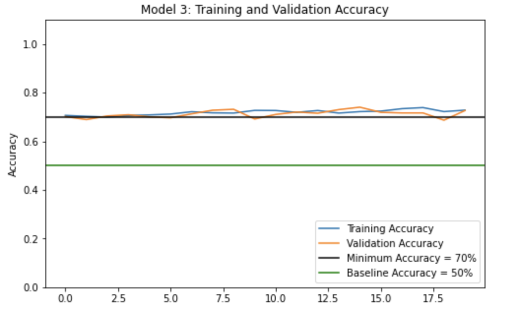
The validation accuracy of the model reaches about 72.54%, in fact it seems to stabilize at around 70-73% during training.

Compared to the validation accuracy obtained in model1 (which was lesser than 70%), this validation accuracy is much higher, which gives us to understand that this model3 does a far better job at classifying cats and dogs than model1.

We notice that the training accuracy and validation accuracy for model3 is quite comparable, there seems to be almost no overfitting! We can safely conclude that model3 is less likely to overfit the data than model1. We should also now that model3 has a more complete, robust data set with artificial transformations of the original images, hence overfitting is less likely to occur.

Part 5: Transfer Learning

Till now, we have been training machine learning models to classify cats and dogs from scratch. While it is indeed worthwhile to know how to train a model from scratch, in this day and age it is highly possible that another individual might have already trained a model to accomplish a very similar task, and perhaps they retrieved meaningful insights or learned some relevant patterns. Since people train machine learning models for a number of image recognition tasks, we could simply use a pre-existing model to classify our cats and dogs! To do so, we will need to first access a pre-existing “base model”, incporate this “base model” into a full model to classify our cats and dogs, and then train that model.

Running the following lines of code will download MobileNetV2 (a feature extractor used for object detection or segmentation) and configure it as a layer, which can then be included within our model.

IMG_SHAPE = IMG_SIZE + (3,)
base_model = tf.keras.applications.MobileNetV2(input_shape=IMG_SHAPE,
                                               include_top=False,
                                               weights='imagenet')
base_model.trainable = False

i = tf.keras.Input(shape=IMG_SHAPE)
x = base_model(i, training = False)
base_model_layer = tf.keras.Model(inputs = [i], outputs = [x])

Now, we will create model4 using MobileNetV2, as follows:

model4 = tf.keras.Sequential([
    # Preprocessor
    preprocessor,
    # Data Augmentation
    layers.RandomFlip("horizontal_and_vertical"),
    layers.RandomRotation(0.25),

    # Base model 
    base_model_layer,
    layers.GlobalMaxPooling2D(),
    layers.Dropout(0.2),
    layers.Dense(1)
])

Now, let’s take a look at our model summary to see how complex the base_model_layer really is!

model4.summary()

Model: "sequential_1"
_________________________________________________________________
Layer (type)                Output Shape              Param #   
=================================================================
model (Functional)          (None, 160, 160, 3)       0         
                                                             
random_flip_2 (RandomFlip)  (None, 160, 160, 3)       0         
                                                             
random_rotation_2 (RandomRo  (None, 160, 160, 3)      0         
tation)                                                         
                                                             
model_1 (Functional)        (None, 5, 5, 1280)        2257984   
                                                             
global_max_pooling2d (Globa  (None, 1280)             0         
lMaxPooling2D)                                                  
                                                             
dropout_2 (Dropout)         (None, 1280)              0         
                                                             
dense_3 (Dense)             (None, 1)                 1281      
                                                             
=================================================================
Total params: 2,259,265
Trainable params: 1,281
Non-trainable params: 2,257,984
_________________________________________________________________

Wow! We only have to train 1,281 parameters in this model - this is so much lower than the number of parameters we had to train for model1 (i.e., upwards of 56,000 parameters).

Finally, let’s compile our model and plot its history of accuracy! We are hoping for a validation accuracy of 95%!

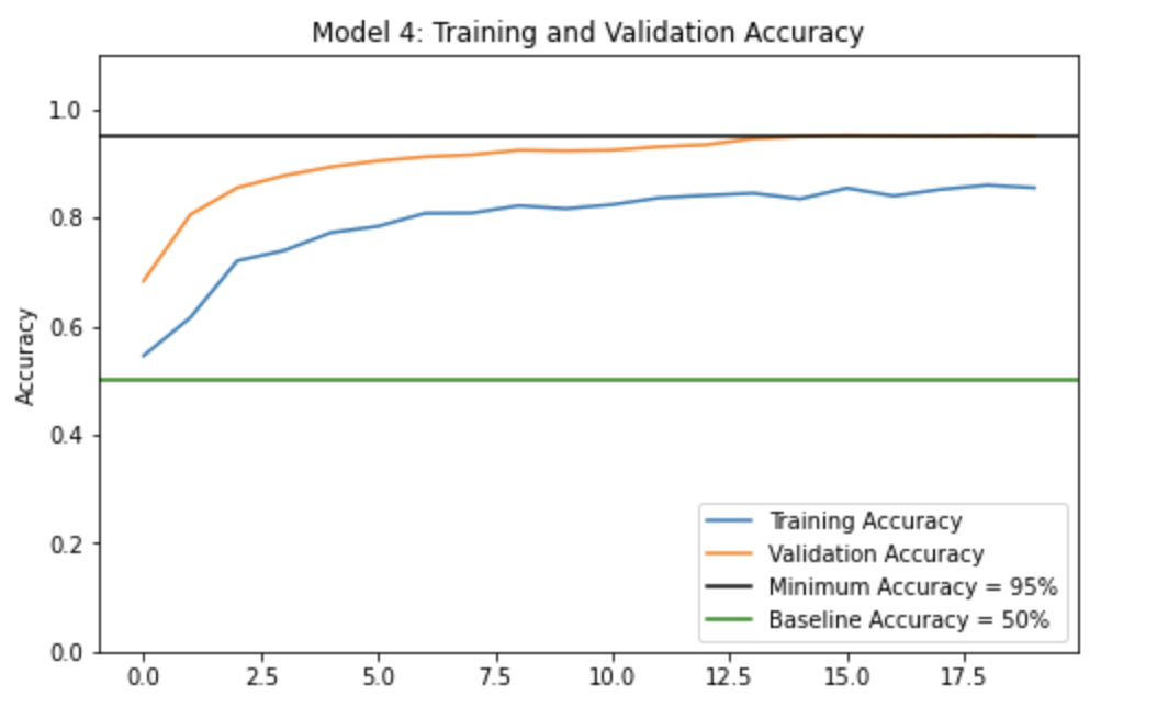
The validation accuracy for this model stabilizes around 94.55% to 95.20% after about 13 epochs!

This validation accuracy (~95%) is so much higher than the validation accuracies for Models 1, 2, and 3! It is clear that this model seems much better at classifying cats and dogs.

Since the training accuracy is always lower than the validation accuracy, safe to say that there is no overfitting!

Part 6: Score on Test Data

Finally, let us evaluate the accuracy of our most performant model, i.e., model4, on the unseen test_dataset and see how we do!

model4.evaluate(test_dataset)

6/6 [==============================] - 1s 70ms/step - loss: 0.0401 - accuracy: 0.9688
[0.04010375216603279, 0.96875]

That’s awesome! Our accuracy is 96.88%!! We can be sure that this model (model4) will do very well at distinguishing between cats and dogs (at least 96.88% of the time).

It turns out that MobileNetV2 made the model a lot better, however it took a little bit longer to train. Perhaps this is because of the complexity of the model (we saw in our model summary that it was pretty complex)!

Congratulations, you did it!!!