This blog post was created for my PIC16B class at UCLA (Previously titled: Blog Post 4 - An Intro to Spectral Clustering).

In this blog post, I’ll be outlining how we might execute the the spectral clustering algorithm for clustering data points.

The source code for this blog post was taken from a Jupyter Notebook written by Dr. Phil Chodrow which can be accessed at this link.

Clustering is a type of unsupervised machine learning task and is a particularly popular technique for exploratory data analysis. The goal of clustering is to divide unlabelled data into groups such that the data points that are most similar to each other are assigned to the same group.

The Spectral Clustering algorithm has become more popular on account of its speedy performance and simple implementation. This technique was dervied using principles of graph theory - i.e., the underlying methodology involves identifying communities of nodes based on the edges connecting them in a given graph. This clustering method can be used to determine the meaningful parts of data sets with complex structures, thereby allowing us to cluster non-graph data too!

Before we dive into spectral clustering, let’s look at an example where we do not require spectral clustering. Let’s go ahead and import the required packages - numpy, sci-kit learn, and matplotlib.

# Importing the relevant packages
import numpy as np
from sklearn import datasets
from matplotlib import pyplot as plt

Note that we will be using the sklearn.datasets package to assign data to the \(\mathbf{X}\) and \(\mathbf{y}\) variables (where \(\mathbf{X}\) contains the Euclidean coordinates of the data points and \(\mathbf{y}\) contains the labels of the data). We will visualize our data in a scatter plot!

n = 200
np.random.seed(1111)
X, y = datasets.make_blobs(n_samples=n, shuffle=True, random_state=None, centers = 2, cluster_std = 2.0)
# Let's visualize our data
plt.scatter(X[:,0], X[:,1])

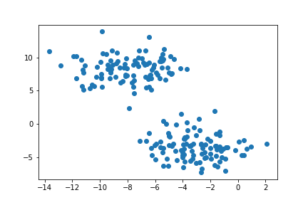
Recall that the goal of clustering is to divide unlabelled data into its natural groups or “blobs”. From the above plot we can already see two natural clusters; we want an algorithm to group our unlabelled data accordingly. The K-Means algorithm is a very popular method to achieve this. So, let’s go ahead and import K-Means into Python from the sklearn.cluster library.

from sklearn.cluster import KMeans
# Since we have two natural clusters, we can declare it here!
km = KMeans(n_clusters = 2)
km.fit(X)

# Visualizing our data after clustering
plt.scatter(X[:,0], X[:,1], c = km.predict(X))

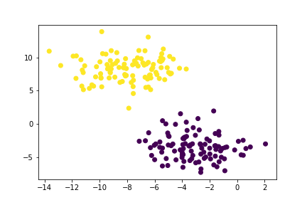
So, we’ve successfully grouped our unlabelled data points into clusters. But what happens when our data is shaped weirdly, i.e., not “blobs”?

np.random.seed(1234)
n = 200
X, y = datasets.make_moons(n_samples=n, shuffle=True, noise=0.05, random_state=None)
# Let's visualize our weirdly shaped data
plt.scatter(X[:,0], X[:,1])

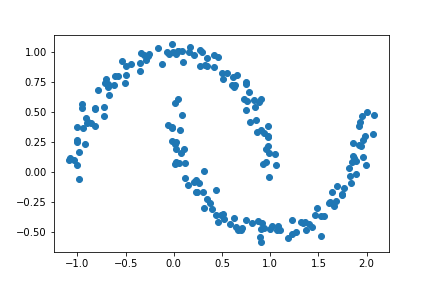
Just by looking at the above plot, we note that we still have two clusters in our data, it’s just that now they are not “blobs” but cresent moons. Let’s go ahead and try implementing our K-Means Algorithm to this data!

km = KMeans(n_clusters = 2)
km.fit(X)
plt.scatter(X[:,0], X[:,1], c = km.predict(X))

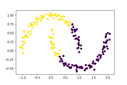
You might notice that this algorithm doesn’t do a very good job and dividing the data points into their natural clusters. This is because the K-Means algorithm looks for circular or blob-like clusters and hence won’t work as well with this cresent-shaped data.

So how can we correctly cluster this data? Through spectral clustering of course!

Before we begin, a little note on syntax:

• Bold uppercase letters (e.g., \(\mathbf{A}\)) signify matrices (i.e., 2d np.ndarray).
• Bold lowercase letters (e.g. \(\mathbf{v}\)) signify vectors (i.e., 1d np.ndarray)
• The matrix-matrix product (i.e., A @ B) is given the notation \(\mathbf{AB}\).
• The matrix-vector product (i.e., A @ v) is given the notation \(\mathbf{Av}\).

Part A: The Similarity Matrix

The first step in our spectral clustering algorithm is to construct our similarity matrix, \(\mathbf{A}\). Similarity matrix \(\mathbf{A}\) must have the shape \((n, n)\) for \(n\) number of data points. We will use a parameter \(\varepsilon\) to construct \(\mathbf{A}\).

Let \(A_{ij}\) correspond to the element of matrix \(\mathbf{A}\) at the \(i\)th row and \(j\)th column for \(1\leq i, j\leq n\). Also let \(X_{k}\) correspond to the coordinates of some data point \(k\) (i.e., the \(k\)th data point in \(\mathbf{X}\)) such that \(1\leq k\leq n\).

Then, we assign values to our matrix \(\mathbf{A}\) such that the following condition is met.

• If the coordinates of some data point \(i\) are within \(\varepsilon\) distance of the coordinates of data point \(j\), then we set the corresponding element \(A_{ij}\) to 1.
  In equation form, \(A_{ij}\) = 1 if \((X_i - X_j)^2 < \varepsilon^2\) for \(1\leq i, j\leq n\)
• If the coordinates of some data point \(i\) are not within \(\varepsilon\) distance of the coordinates of data point \(j\), then we set the corresponding element \(A_{ij}\) to 0.
  In equation form, \(A_{ij}\) = 0 if \((X_i - X_j)^2 \geq \varepsilon^2\) for \(1\leq i, j\leq n\)
• All diagonal entries \(A_{ii}\) should all be equal to zero.
  In equation form, \(A_{ij}\) = 0 whenever \(i = j\)

Let us set \(\varepsilon = 0.4\).

epsilon = 0.4

We already have our the coordinates of our data points stored in X and our labels in y. We also have the number of data points stored in n. Let’s check these variables!

X.shape, y.shape, n

((200, 2), (200,), 200)

While constructing our matrix \(\mathbf{A}\), we could use for-loops to manually iterate through the elements of our matrix and set them to 0 or 1 accordingly. However, we could also use this really handy built in solution from sklearn!

from sklearn.metrics.pairwise import pairwise_distances
# Function computes all the pairwise distances!
A = pairwise_distances(X, X)
A.shape # checking A to make sure it has (n, n) shape. 

(200, 200)

The pairwise_distances function computes all the pairwise distances and collects them into an appropriate matrix. Isn’t this so much easier than manually looping through all the elements?!

Let’s take a look at a 5x5 slice of our matrix \(\mathbf{A}\).

A[:5, :5]

array([[0.        , 1.27292462, 1.33315598, 1.97506495, 2.43337261],
       [1.27292462, 0.        , 1.46325112, 1.93152405, 2.18793876],
       [1.33315598, 1.46325112, 0.        , 0.64238147, 1.10996726],
       [1.97506495, 1.93152405, 0.64238147, 0.        , 0.50493603],
       [2.43337261, 2.18793876, 1.10996726, 0.50493603, 0.        ]])

We note that matrix \(\mathbf{A}\) currently stores the exact pairwise distances instead of 0s or 1s. Therefore, we need to replace all elements that are less than \(\varepsilon\) with 1 and all other elements with 0. Thankfully, we have a very handy np.where function that allows us to do just that!

A = np.where(A < epsilon, 1, 0)
# Checking the 5x5 slice of matrix A
A[:5, :5]

array([[1, 0, 0, 0, 0],
       [0, 1, 0, 0, 0],
       [0, 0, 1, 0, 0],
       [0, 0, 0, 1, 0],
       [0, 0, 0, 0, 1]])

Finally, we have to make sure that all elements along the diagonal of matrix \(\mathbf{A}\) are set to 0. We can use the np.fill_diagonal function to accomplish this!

np.fill_diagonal(A, 0)
# Checking a 5x5 slice of matrix A
A[:5, :5]

array([[0, 0, 0, 0, 0],
       [0, 0, 0, 0, 0],
       [0, 0, 0, 0, 0],
       [0, 0, 0, 0, 0],
       [0, 0, 0, 0, 0]])

Notice how all the 1s along the diagonal have turned into 0s? Congratulations! We’ve finished constructing our similarity matrix \(\mathbf{A}\)!

Part B: The Binary Norm Cut Objective of the Similarity Matrix

Our similarity matrix \(\mathbf{A}\) contains information about which data points lie within \(\varepsilon\) distance of other data points points. We will now attempt to partition the rows and columns of \(\mathbf{A}\).

Before we define the binary norm cut objective function, let’s first define a couple of things. First we define the \(i\)th row sum of \(\mathbf{A}\) or the degree of \(i\) as follows: \[d_i = \Sigma_{j=1}^n A_{ij}\] Also let \(C_0\) and \(C_1\) be clusters of data points. We will assume that all of the \(n\) data points will either belong to \(C_0\) or \(C_1\). Our clustering vector \(\mathbf{y}\) will tell us which cluster a data point belongs to, i.e., \(y_i\) tells us the cluster membership of data point \(i\) whose coordinates are given by \(X_i\). If \(y_i = 1\), then point \(i\) belongs to cluster \(C_1\). Similarly, if \(y_i = 0\), then point \(i\) belongs to cluster \(C_0\).

Now that we’ve established the above, let’s define our binary norm cut objective function: \[N_A(C_0, C_1) \equiv \mathbf{cut}(C_0, C_1)\left(\frac{1}{\mathbf{vol}(C_0)} + \frac{1}{\mathbf{vol}(C_1)} \right)\]

When \(N_A(C_0, C_1)\) is small, we consider the pair of clusters \(C_0\) and \(C_1\) to be a “good” partition of the data. To understand why this is true, we will need to look at the two factors in this function: \(\mathbf{cut}\) and \(\mathbf{vol}\).

Part B.1 The Cut Term

Let’s first take a look at the cut of the clusters \(C_0\) and \(C_1\) that is given by: \[\mathbf{cut}(C_0, C_1) \equiv \Sigma_{i\in C_0, j\in C_1} A_{ij}\]

The cut term \(\mathbf{cut}(C_0, C_1)\) corresponds to the number of non-zero entries in \(\mathbf{A}\) that relate data points in \(C_0\) to data points in \(C_1\). So, if the cut term is small, it follows that the points in cluster \(C_0\) will not be very close to the points in cluster \(C_1\).

We will now define a function cut(A, y) that computes the cut term using the above formula.

def cut(A, y):
    """
    Function computes the cut term by summing up the entries A[i,j] 
    for each pair of data points (i,j) in different clusters.

    Parameters
    ----------
    A : 2d np.ndarray
        The similarity matrix
    y : 1d np.ndarray
        The labels of the data

    Returns 
    ----------
    int
        The cut term
    """
    sum = 0
    for i in range(n):
        for j in range(n):
            # from the above formula
            # point i must be in cluster C_0
            # point j must be in cluster C_1
            if (y[i] == 0) and (y[j] == 1):
                sum += A[i][j]
    return sum

Now that we’ve written out cut(A, y) function, we will use it to compute the cut objective for the true clusters y.

# using our previously defined A and y
cut(A, y)

13

Now, we will generate a random vector of size n with random labels (that are either 0 or 1). We want to check the cut term for these random labels. If we have written our function correctly, we should find that the cut objective for these random labels is much larger than the cut objective for the true labels.

# Choosing random labels 0, 1 for a vector of size n
random_labels = np.random.randint(2, size=n)

# Checking the cut term
cut(A, random_labels)

1150

Hooray! We’ve successfully shown that the cut objective for these random labels is much larger than the cut objective for the true labels!

Part B.2 The Volume Term

The volume of some cluster \(C_k\) where \(k = 0, 1\) is a measure of the size of that cluster. We can compute the volume term using the following: \[ \mathbf{vol}(C_k) \equiv \Sigma_{i\in C_k} d_i \] where \(d_i\) is the degree of row \(i\) and \(k = 0, 1\).

Notice that if we assume a cluster \(C_k\) is small, then it follows that \(\mathbf{vol}(C_k)\) would be small and hence, the inverse \(\frac{1}{\mathbf{vol}(C_k)}\) would be large. This is undesirable as it would lead to a higher objective value (which we do not want since we want the binary norm cut objective to be small).

Therefore, we need to find clusters \(C_0\) and \(C_1\) such that: (1) There are relatively few entries of \(\mathbf{A}\) that relate data points in \(C_0\) to data points in \(C_1\), and (2) Clusters \(C_0\) and \(C_1\) are not too small.

Let’s write a function vols(A, y) that computes the volumns of both \(C_0\) and \(C_1\).

def vols(A, y):
    """
    Function computes the volumes of C_0 and C_1 using 
    the above formula, returning them as a tuple. 
    
    Parameters
    ----------
    A : 2d np.ndarray
        The similarity matrix
    y : 1d np.ndarray
        The labels of the data

    Returns
    ----------
    tuple
        The volumes of cluster C_0 and C_1
    """
    # volume of cluster C_0
    vol_c0 = np.sum([np.sum(A[i]) for i in range(n) if y[i] == 0])
    # volume of cluster C_1
    vol_c1 = np.sum([np.sum(A[i]) for i in range(n) if y[i] == 1])

    return (vol_c0, vol_c1)

Now that we have defined our cut(A, y) and vols(A, y) functions, we can compute the binary normalized cut objective of matrix \(\mathbf{A}\) with the clustering vector \(\mathbf{y}\). Let’s write a function called normcut(A, y) that does this for us!

def normcut(A, y):
    """
    Function computes the binary normalized cut 
    objective of a matrix A with clustering vector y.

    Parameters
    ----------
    A : 2d np.ndarray
        The similarity matrix
    y : 1d np.ndarray
        The labels of the data (clustering vector)
    
    Returns
    ----------
    float
        The binary normalized cut objective
    """
    # computing the volumes
    volC0, volC1 = vols(A, y)
    # computing the norm cut
    norm = cut(A, y)*((1/volC0)+(1/volC1))
    return norm

Now, we will compare the normcut objective using the true labels \(\mathbf{y}\) and the random labels we generated earlier! We should observe that the normcut objective for the true labels is far smaller since this would indicate a better partition of the data!

# Normcut for true labels
normcut(A, y)

0.011518412331615225

# Normcut for random labels
normcut(A, random_labels)

1.0240023597759158

We note that the normcut for the true labels \(\mathbf{y}\) is significantly smaller (about a hundred times smaller) than the normcut for the random labels!

Part C: Minimizing the Normcut Objective

Now that we have our function normcut(A, y), one possible approach to this clustering problem is to find a vector \(\mathbf{y}\) such that normcut(A, y) is minimized. However, it may not be possible to find the clustering in practical time if we attempt to solve this optimization problem. We will need to use a math trick to solve this!

We will define a new vector \(\mathbf{z}\in\mathbb{R}^n\) such that:

• \(z_i = \frac{1}{\mathbf{vol}(C_0)}\) if \(y_i = 0\)
• \(z_i = -\frac{1}{\mathbf{vol}(C_1)}\) if \(y_i = 1\)

We note that the signs of the elements of \(\mathbf{z}\) contain the information from our clustering vector \(\mathbf{y}\). For instance, if data point \(i\) is in cluster \(C_0\), we know that \(y_i = 0\) and \(z_i > 0\). Similarly, if data point \(i\) is in cluster \(C_1\), we know that \(y_i = 1\) and \(z_i < 0\).

Let’s write a function called transform(A, y) to construct the vector \(\mathbf{z}\) using the conditions specified above.

def transform(A, y):
    """
    Function computes appropriate z vector using the above formula

    Parameters
    ----------
    A : 2d np.ndarray
        The similarity matrix
    y : 1d np.ndarray
        The labels of data (clustering vector)

    Returns
    ----------
    np.ndarray
        The z vector
    """
    # extracting the volumes of clusters
    volC0, volC1 = vols(A, y)
    # computing the n-dimensional vector z
    z = np.where(y == 0, 1/volC0, (-1)/volC1)
    return z

Now that we have written our transform(A, y) function that helps us contruct vector \(\mathbf{z}\), we want to show that \[\mathbf{N_A}(C_0, C_1) = \frac{\mathbf{z}^T(\mathbf{D} - \mathbf{A})\mathbf{z}}{\mathbf{z}^T\mathbf{D}\mathbf{z}}\] where \(\mathbf{D}\) is a diagonal matrix with non-zero entries such that \(d_{ii} = d_i\) for some \(1\leq i\leq n\). Recall that \(d_i\) is the degree of row \(i\) in matrix \(\mathbf{A}\).

We want to check that this equation relates the matrix product to the normcut objective. Let’s compute the left hand side (lhs) and right hand side (rhs) of the equations seperately and check whether they are approximate.

# computing left hand side of equation
lhs = normcut(A, y)

# computing right hand side of equation

# diagonal matrix
D = np.diag(np.sum(A, axis=0))
# vector z
z = transform(A, y)
# right hand side 
rhs = (z @ (D - A) @ z)/(z @ D @ z)

Now, we can use our handy np.isclose function to see whether lhs is close to rhs. Remember, we want our np.isclose function to return True!

# Checking whether the right and left and side values
# are approximate
np.isclose(lhs, rhs)

True

Consider the identity \(\mathbf{z}^T\mathbf{D}\mathbb{1} = 0\) where \(\mathbb{1}\) is an array of 1s with size \(n\). If this identity holds true, it tells us that vector \(\mathbf{z}\) has as many positive entries as it does negative ones.

# Checking the identity  𝐳.T @ 𝐃 @ 𝟙 = 0

# array of ones
arr_ones = np.ones(n)
# computing the identity
identity = z.T @ D @ arr_ones

# checking if identity is close to 0
np.isclose(identity, 0)

True

Part D: Explicit Optimization

From the last part, we have seen that minimizing the normcut objective is mathematically related to minimizing the following function with respect to \(\mathbf{z}\): \[R_A(\mathbf{z}) = \frac{\mathbf{z}^T(\mathbf{D} - \mathbf{A})\mathbf{z}}{\mathbf{z}^T\mathbf{D}\mathbf{z}} \qquad \text{subject to} \qquad \mathbf{z}^T\mathbf{D}\mathbb{1} = 0\]

It is possible to incorporate this condition (i.e., \(\mathbf{z}^T\mathbf{D}\mathbb{1} = 0\)) into the optimization problem by substituting the orthogonal complement of \(\mathbf{z}\) relative to \(\mathbf{D}\mathbb{1}\) in place of \(\mathbf{z}\). The following orth_obj function handles this:

def orth(u, v):
    return (u @ v) / (v @ v) * v

e = np.ones(n)

d = D @ e 

def orth_obj(z):
    z_o = z - orth(z, d)
    return (z_o @ (D - A) @ z_o)/(z_o @ D @ z_o)

Now, let’s go ahead and use our handy minimize function from the scipy.optimize library to minimize the orth_obj function with respect to \(\mathbf{z}\). Note that our minimize function requires two inputs: (1) the objective function to be minimized and (2) the initial guess array which is set to what we think the minimum is close to (I’ve initialized init_guess to an array of ones). Let’s call our minimizing vector z_min.

In Part C, we made sure the entries of \(\mathbf{z}\) were only 0 or 1, however now we are allowing the entries of \(\mathbf{z}\) to take on any value. So, instead of optimizing the exact normcut objecting, we’re optimizing an approximation of the function! This is the continuous relaxation of the normcut problem!

import scipy.optimize as so

init_guess = np.full(len(z), 1) # array of ones as our initial guess
# extracting the minimum vecctor
z_min = so.minimize(orth_obj, init_guess).x

Part E: Results of Explicit Optimization

Recall that our vector \(\mathbf{z}\) carries the information stored in \(\mathbf{y}\)! If data point \(i\) is in cluster \(C_0\), we know that \(y_i = 0\) and \(z_i > 0\). Similarly, if data point \(i\) is in cluster \(C_1\), we know that \(y_i = 1\) and \(z_i < 0\).

Let’s plot the original data, using one color for points such that z_min[i] < 0 and another color for all other values of z_min that do not satisfy the aforementioned condition.

# Where z_min[i] < 0, we have label 1
# Where z_min[i] >= 0, we have label 0
labels = np.where(z_min < 0, 1, 0) 

# Plotting the original data
plt.scatter(X[:,0], X[:,1], c = labels)

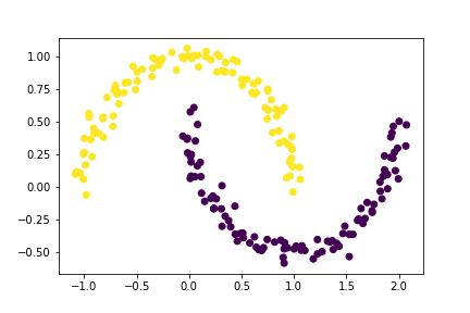
Wow! It does look like we were able to cluster this data pretty well!

Part F: Spectral Clustering

You might have noticed that it took a while for z_min to be computed. This is because explicit optimization can be quite slow (even if it does get the job done). Spectral clustering is much faster!

Spectral clustering, as the name suggests, involves using the eigenvalues and eigenvectors from matrices to solve the same optimization problem we saw in Part D and E. Recall that we wanted to minimize the following function with respect to \(\mathbf{z}\): \[R_A(\mathbf{z}) \equiv \frac{\mathbf{z}^T(\mathbf{D}-\mathbf{A})\mathbf{z}}{\mathbf{z}^T\mathbf{D}\mathbf{z}} \qquad \text{subject to} \qquad \mathbf{z}^T\mathbf{D}\mathbb{1} = 0\]

Consider the Rayleigh-Ritz Theorem which states that a minimizing \(\mathbf{z}\) must be the solution of the generalized eigenvalue problem (\(1\)) with the smallest eigenvalue : \[(\mathbf{D}-\mathbf{A})\mathbf{z} = \lambda\mathbf{D}\mathbf{z}, \qquad \mathbf{z}^T\mathbf{D}\mathbb{1} = 0 \qquad \cdots(1)\] (\(1\)) happens to be equivalent to the standard eigenvalue problem (\(2\)): \[\mathbf{D}^{-1}(\mathbf{D}-\mathbf{A})\mathbf{z} = \lambda\mathbf{z}, \qquad \mathbf{z}^T\mathbf{D}\mathbb{1} = 0 \qquad \cdots(2)\]

This is helpful for us to know because \(\mathbb{1}\) happens to be the eigenvector corresponding to the smallest eigenvalue of the matrix \(\mathbf{D}^{-1}(\mathbf{D}-\mathbf{A})\). Therefore, the \(\mathbf{z}\) vector we would like to determine must be the eigenvector corresponding to the second-smallest eigenvalue.

Therefore, we must first construct the normalized Laplacian matrix, \(\mathbf{L} = \mathbf{D}^{-1}(\mathbf{D}-\mathbf{A})\) of the similarity matrix \(\mathbf{A}\) and extract its eigenvalues and corresponding eigenvectors. Then, we must retrieve the eigenvector corresponding to the second-smallest eigenvalue. We will call this eigenvector z_eig.

# Constructing the normalized Laplacian matrix (L)
L = np.linalg.inv(D) @ (D - A)

# Extracting the eigenvalues and eigenvectors of L
eigvalues, eigvectors = np.linalg.eig(L)
# We want to find the eigenvector corresponding to the 
# second smallest eigenvalue
sorted_values = eigvalues[np.argsort(eigvalues)]
sorted_vectors = eigvectors[:, np.argsort(eigvalues)]
# vector corresponding to 2nd smallest eigenvector
z_eig = sorted_vectors[:, 1] 

Now that we have retrieved our z_eig vector, we can go ahead and plot the data again while using the signs of the entries of z_eig to assign different colors to each data point (similar to what we did in Part E).

# Where z_eig[i] < 0, we have label 1
# Where z_eig[i] >= 0, we have label 0
labels_new = np.where(z_eig < 0, 1, 0) 

# Plotting the original data
plt.scatter(X[:,0], X[:,1], c = labels_new)

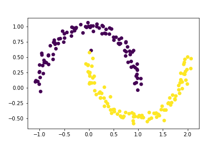
Looks like our algorithm worked pretty well! There appears to be only one data point that is incorrectly clustered!

Though the clusters after the explicit optimization seem to be a little more accurate (i.e., there were no visible incorrectly clustered points), spectral clustering was so much faster! Thus, even though there seems to be one data point that is incorrectly clustered this method is exceedingly fast and also accurate to a very high degree, which is what makes it very popular!

Part G: Synthesizing the Results

Now let’s combine everything that we’ve done so far into one function spectral_clustering(X, epsilon) which takes in the input data \(\mathbf{X}\) (the Euclidean coordinates of the data points) and the distance threshold \(\varepsilon\). The function should perform spectral clustering and return an array of binary labels, indicating the cluster that a data point belongs to, i.e., whether a particular data point is in group 0 or group 1 (cluster \(C_0\) or \(C_1\)).

def spectral_clustering(X, epsilon):
    """
    Function performs spectral clustering for clustering
    data points
    
    Parameters
    ----------
    X : np.ndarray
        The array of input data
    epsilon : float
        The distance threshold
        
    Returns
    ----------
    array
        Function returns an array of binary labels
        indicating whether data point i is in group
        0 or group 1
    """
    # 1 - Constructing the similarity matrix A
    A = pairwise_distances(X, X) 
    A = np.where(A < epsilon, 1, 0)
    np.fill_diagonal(A, 0)
    
    # 2 - Constructing the Laplacian matrix L
    D = np.diag(np.sum(A, axis=0)) # diagonal array
    L = np.linalg.inv(D) @ (D - A)
    
    # 3 - Compute the eigenvector with second-smallest 
    #     eigenvalue of the Laplacian matrix.
    evals, evecs = np.linalg.eig(L)
    sorted_vecs = evecs[:, np.argsort(evals)]
    z_eig = sorted_vecs[:, 1]
    
    # 4 - Return labels based on z_eig
    labels = np.where(z_eig < 0, 1, 0) 
    
    return labels

Let’s go ahead and test our function!

# extracting the labels
spectral_labels = spectral_clustering(X, epsilon)

# Plotting the data
plt.scatter(X[:,0], X[:,1], c = spectral_labels)

It looks like our function works!

Notice how easy it was to implement this function? The function in itself is very compact (exactly ten lines of code if you ignore the comments and the docstrings). So, not only is the compute time for this function very small, it is also very easy to implement. Thus, even though there seems to be one data point that is incorrectly clustered, this ease with which this algorithm can be implemented along with the small compute time makes it very popular!

Part H: A Few More Experiments…

Let’s go ahead and run a few more experiments using our new spectral_clustering function! We will generate different data sets while increasing the noise to see what effect it has on the clustering of data points!

Experiment H.1

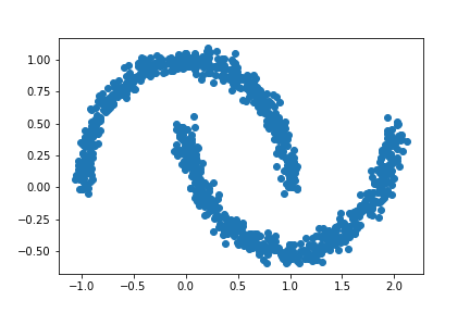
For this experiment, let noise = 0.05.

n = 1000 # number of data points
# Creating a new data set
X, y = datasets.make_moons(n_samples=n, shuffle=True, noise=0.05, random_state=None)

# Plotting the data set
plt.scatter(X[:,0], X[:,1])

# Applying our clustering algorithm
# extracting the labels
labels = spectral_clustering(X, epsilon)
# Plotting the data
plt.scatter(X[:,0], X[:,1], c = labels)

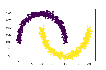
So, our algorithm worked pretty well for this case. Let’s go ahead and increase our noise in the next experiment to see what happens!

Experiment H.2

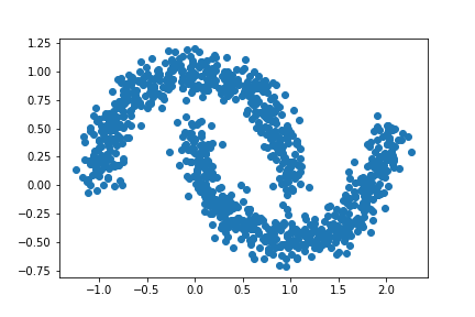
Let us increase our noise. For this experiment, let the noise = 0.10.

n = 1000 # number of data points
# Creating a new data set
X, y = datasets.make_moons(n_samples=n, shuffle=True, noise=0.10, random_state=None)

# Plotting the data set
plt.scatter(X[:,0], X[:,1])

# Applying our clustering algorithm
# extracting the labels
labels = spectral_clustering(X, epsilon)
# Plotting the data
plt.scatter(X[:,0], X[:,1], c = labels)

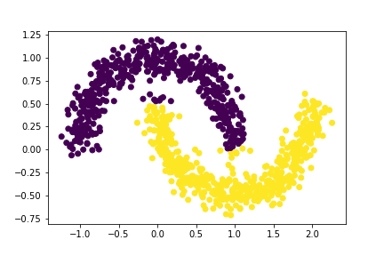
As we can see, our data set is a little more noisy, however our spectral clustering algorithm still seems to be working pretty well with only a few points that are misclustered. Let’s go ahead and increase it further to see what will happen!

Experiment H.3

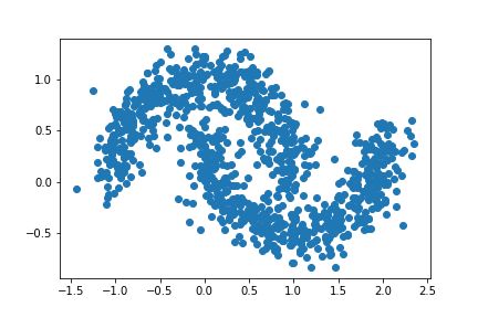
Let us increase our noise even more. For this experiment, let the noise = 0.15.

n = 1000 # number of data points
# Creating a new data set
X, y = datasets.make_moons(n_samples=n, shuffle=True, noise=0.15, random_state=None)

# Plotting the data set
plt.scatter(X[:,0], X[:,1])

# Applying our clustering algorithm
# extracting the labels
labels = spectral_clustering(X, epsilon)
# Plotting the data
plt.scatter(X[:,0], X[:,1], c = labels)

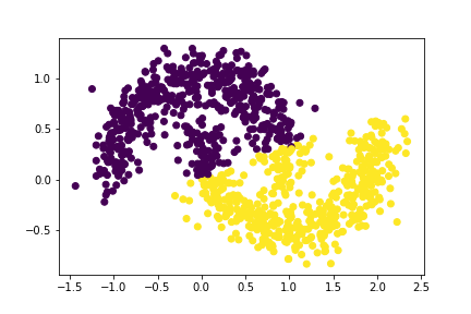
Oops! This doesn’t look to good! There seem to be a significant number of data points that are incorrectly clustered. It appears that the algorithm doesn’t seem to work as well in seperating the data points into their natural clusters.

Experiment H.4

We will increase our noise one last time. For this experiment, let noise = 0.20.

n = 1000 # number of data points
# Creating a new data set
X, y = datasets.make_moons(n_samples=n, shuffle=True, noise=0.20, random_state=None)

# Plotting the data set
plt.scatter(X[:,0], X[:,1])

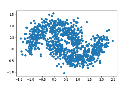
# Applying our clustering algorithm
# extracting the labels
labels = spectral_clustering(X, epsilon)
# Plotting the data
plt.scatter(X[:,0], X[:,1], c = labels)

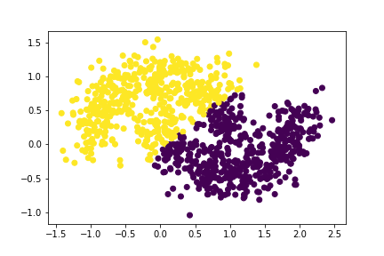
Oops! This looks even worse than the clusters for our previous experiment. We notice that the algorithm doesn’t seem to work as well in seperating the data points into their natural clusters.

Therefore, we can safely conclude that as the noise is increased, it is likely that the effectiveness of our spectral clustering algorithm would decrease.

Part I: Some More Experiments…

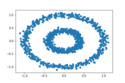
Let’s try testing our spectral_clustering function with another type of data set. Our new data will be bull’s eye shaped (i.e., there will be two concentric circles).

n = 1000
X, y = datasets.make_circles(n_samples=n, shuffle=True, noise=0.05, random_state=None, factor = 0.4)
plt.scatter(X[:,0], X[:,1])

Let’s try clustering our new data with K-Means!

km = KMeans(n_clusters = 2)
km.fit(X)
plt.scatter(X[:,0], X[:,1], c = km.predict(X))

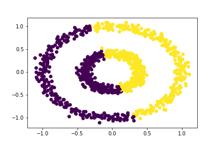
Similar to our crescent moon data, we noticed that the K-Means algorithm will not work as well in seperating these points into their natural clusters. This is because the K-Means algorithm looks for blob-like clusters to seperate data points into their clusters.

Let’s now attempt to cluster our data with the spectral_clustering function. We will attempt to find the clustering for various values of \(\varepsilon\), such that \(0 < \varepsilon < 1\).

Experiment I.1

Let our distance threshold, \(\varepsilon = 0.2\).

# Applying our clustering algorithm
epsilon = 0.2
# extracting the labels
c_labels = spectral_clustering(X, epsilon)
# Plotting the data
plt.scatter(X[:,0], X[:,1], c = c_labels)

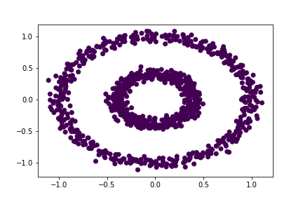
Notice that our clustering algorithm put all of our data into the same cluster! This might imply that our current distance threshold is too small!

Experiment I.2

Let our distance threshold, \(\varepsilon = 0.4\).

# Applying our clustering algorithm
epsilon = 0.4
# extracting the labels
c_labels = spectral_clustering(X, epsilon)
# Plotting the data
plt.scatter(X[:,0], X[:,1], c = c_labels)

We notice that our clustering algorithm works really well at seperating the data points into their natural clusters for this \(\varepsilon\) value!

Experiment I.3

Let our distance threshold, \(\varepsilon = 0.6\).

# Applying our clustering algorithm
epsilon = 0.6
# extracting the labels
c_labels = spectral_clustering(X, epsilon)
# Plotting the data
plt.scatter(X[:,0], X[:,1], c = c_labels)

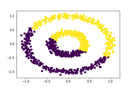
Oops! Our clustering algorithm doesn’t seem to be working too well! In fact, it seems to be working rather the like K-Means algorithm in this case. Perhaps our distance threshold is too large.

Experiment I.4

Let our distance threshold, \(\varepsilon = 0.8\).

# Applying our clustering algorithm
epsilon = 0.8
# extracting the labels
c_labels = spectral_clustering(X, epsilon)
# Plotting the data
plt.scatter(X[:,0], X[:,1], c = c_labels)

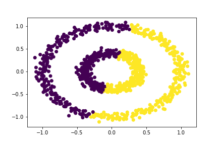
Oops! Just like our previous experiment, our clustering algorithm doesn’t seem to be working too well for this distance threshold either! Perhaps our distance threshold is indeed too large.

Suppose we want to find the values of \(\varepsilon\) for which we can correctly seperate the two rings. We’ve already seen that for a distance threshold of 0.4, our spectral_clustering function seems to be working pretty well, but for a threshold of 0.2 and 0.6 our algorithm doesn’t work as well.

Experiment I.5: Deducing the Minimum Distance Threshold Needed to Correctly Seperate the Two Rings

Experiment I.5.1

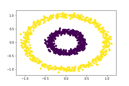
Since we know for sure that our algorithm correctly seperates the two rings for \(\varepsilon = 0.4\), but not for \(\varepsilon = 0.2\), let’s go ahead and see whether our algorithm works correctly for the midpoint of these two thresholds.
Let our distance threshold, \(\varepsilon = 0.3\).

# Applying our clustering algorithm
epsilon = 0.3
# extracting the labels
c_labels = spectral_clustering(X, epsilon)
# Plotting the data
plt.scatter(X[:,0], X[:,1], c = c_labels)

Experiment I.5.2

So, we know that our algorithm correctly seperates the two rings for \(\varepsilon = 0.3\), but not for \(\varepsilon = 0.2\). So, we know that the minimum distance threshold for which the algorithm correctly seperates the two rings must be between 0.2 and 0.3. Let’s check the result for the midpoint once again!

Let our distance threshold, \(\varepsilon = 0.25\).

# Applying our clustering algorithm
epsilon = 0.25
# extracting the labels
c_labels = spectral_clustering(X, epsilon)
# Plotting the data
plt.scatter(X[:,0], X[:,1], c = c_labels)

Experiment I.5.3

Now, we know that our algorithm correctly seperates the two rings for \(\varepsilon = 0.3\), but not for \(\varepsilon = 0.25\). So, we know that the minimum distance threshold must be between 0.25 and 0.3. Let’s check the result for the midpoint once again!

Let our distance threshold, \(\varepsilon = 0.28\).

# Applying our clustering algorithm
epsilon = 0.28
# extracting the labels
c_labels = spectral_clustering(X, epsilon)
# Plotting the data
plt.scatter(X[:,0], X[:,1], c = c_labels)

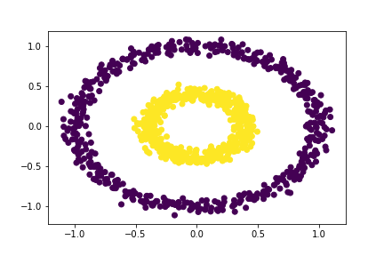
Experiment I.5.3

Our algorithm correctly seperates the two rings for \(\varepsilon = 0.28\), but not for \(\varepsilon = 0.25\). So, we know that the minimum distance threshold must be between 0.25 and 0.28. However, since we only have two options: 0.26 and 0.27, let’s go ahead and simply choose one of those possible distance thresholds.

Let our distance threshold, \(\varepsilon = 0.26\).

# Applying our clustering algorithm
epsilon = 0.26
# extracting the labels
c_labels = spectral_clustering(X, epsilon)
# Plotting the data
plt.scatter(X[:,0], X[:,1], c = c_labels)

Wow! Notice that our algorithm does not correctly seperate the two rings for \(\varepsilon = 0.25\), but correctly seperates the two rings for \(\varepsilon = 0.26\). Therefore, we have deduced the minimum distance threshold needed to correctly seperate the two rings to the second decimal place.

Experiment I.6: Deducing the Maximum Distance Threshold Needed to Correctly Seperate the Two Rings

Experiment I.6.1

We already know that our algorithm correctly seperates the two rings for \(\varepsilon = 0.4\), but not for \(\varepsilon = 0.6\), let’s go ahead and see whether our algorithm works correctly for the midpoint of these two thresholds.
Let our distance threshold, \(\varepsilon = 0.5\).

# Applying our clustering algorithm
epsilon = 0.5
# extracting the labels
c_labels = spectral_clustering(X, epsilon)
# Plotting the data
plt.scatter(X[:,0], X[:,1], c = c_labels)

Experiment I.6.2

We have found that our algorithm correctly seperates the two rings for \(\varepsilon = 0.5\), but not for \(\varepsilon = 0.6\). As a result, we know that the maximum distance threshold must be between 0.5 and 0.6. Let’s go ahead and see whether our algorithm works correctly for the midpoint of these two thresholds.
Let our distance threshold, \(\varepsilon = 0.55\).

# Applying our clustering algorithm
epsilon = 0.55
# extracting the labels
c_labels = spectral_clustering(X, epsilon)
# Plotting the data
plt.scatter(X[:,0], X[:,1], c = c_labels)

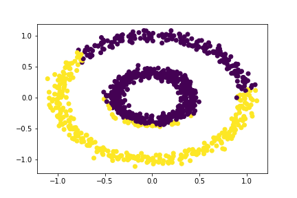
Experiment I.6.3

So, our algorithm correctly seperates the two rings for \(\varepsilon = 0.5\), but not for \(\varepsilon = 0.55\). As a result, we know that the maximum distance threshold must be between 0.5 and 0.55. Let’s go ahead and see whether our algorithm works correctly for the midpoint of these two thresholds.
Let our distance threshold, \(\varepsilon = 0.52\).

# Applying our clustering algorithm
epsilon = 0.52
# extracting the labels
c_labels = spectral_clustering(X, epsilon)
# Plotting the data
plt.scatter(X[:,0], X[:,1], c = c_labels)

Experiment I.6.4

That’s cool! Our algorithm correctly seperates the two rings for \(\varepsilon = 0.52\), but not for \(\varepsilon = 0.55\). So, we know that the maximum distance threshold must be between 0.52 and 0.55. However, since we only have two options: 0.53 and 0.54, let’s go ahead and simply choose one of those possible distance thresholds.

Let our distance threshold, \(\varepsilon = 0.53\).

# Applying our clustering algorithm
epsilon = 0.53
# extracting the labels
c_labels = spectral_clustering(X, epsilon)
# Plotting the data
plt.scatter(X[:,0], X[:,1], c = c_labels)

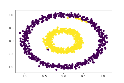
What’s interesting here is that our algorithm seems to be working correctly for the most part — there are only a few data points that seem to be incorrectly clustered. Nonetheless, the maximum distance threshold that correctly clustered all of the data points was \(\varepsilon = 0.52\)

After a series of experiments, we have deduced that the range of epsilon values for which the algorithm is able to correctly seperate the two rings is \(0.26 \leq \varepsilon \leq 0.52\).